The steps of head modeling are segmentation, mesh generation, and co-registration of electrode locations with scalp surface. User may also generate a source space to be used in the solution of the inverse problem. Figure 2 shows the steps of head modeling using MR images.

Each step in realistic head modeling is implemented as a separate GUI module reachable from the main menu. These modules are described in the following sub-sections.

The first step in segmentation is to load the MR image. The input of the segmentation module is a 3-D sagittal T1-weighted MR image. The image format has to be in analyze format and the voxel size need to be 1×1×1 mm. To prepare the image for this toolbox, one may use Freesurfer software (http://surfer.nmr.mgh.harvard.edu/) to perform the following operations:

1. Inhomogeneity correction: mri_nu_correct.mni --i input_volume --o output_volume --n 2

2. Conversion of the input volume to 1 mm volume data: mri_convert -i input_volume --conform_size 1 --o output_volume

3. Orient the image: mri_convert -i input_volume --out_orientation PSR -ot format -o output_volume

4. Save in analyze format: mri_convert -it analyze -i output_file_name.img -ot file_type -o input_volume

When the image is loaded, slices are shown in sagittal, axial, and coronal orientations and it is possible to select slices easily by using the scroll bars or clicking on the images (Figure 3). The Display image panel allows the user to select which image to display on the image panels. The available choices are the MR volume, the filtered volume or various stages of segmentation.

.....

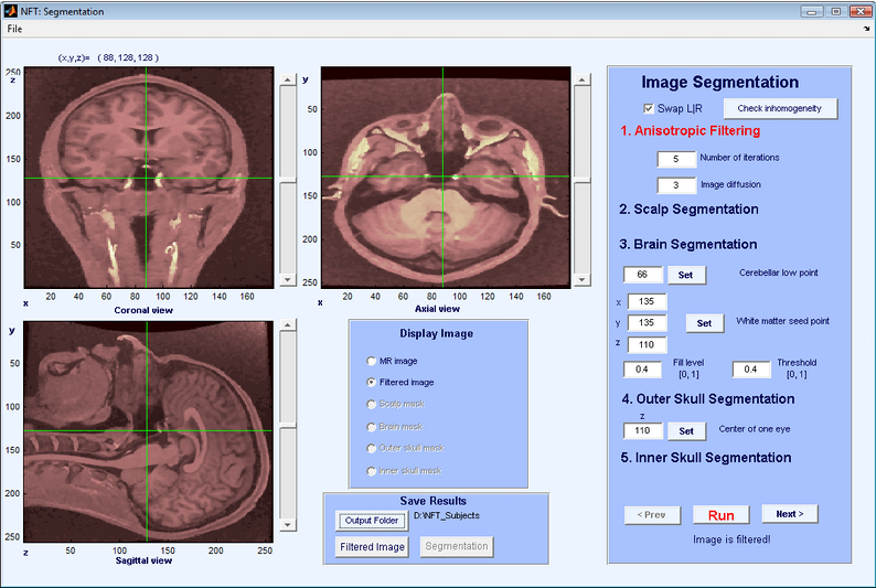
The panel on the right of the segmentation GUI shows the segmentation steps that will be performed on the volume in order:

1. Anisotropic filtering.

2. Scalp segmentation.

3. Brain segmentation.

4. Outer skull segmentation.

5. Inner skull segmentation.

The current step is highlighted in red. Pressing the Run button executes the segmentation step. It is possible to repeat a given step, changing parameters and observing the output. Pressing the Next button proceeds to the next step. Below is a discussion of each segmentation step:

The purpose of anisotropic filtering is to enhance the image quality. This filter increases the SNR of the image while preserving the edges. The inputs to the anisotropic filtering are the number of iterations and image diffusion. The default values of 5 and 3 work well for most MR images. As the values increase, the image starts to get blurred. The output of anisotropic filtering can be observed by selecting “Filtered Image” from the Display Image panel.

The next step is scalp segmentation, separating the background from the image. There are no user inputs to scalp segmentation. An automatic thresholding algorithm is applied, and the result can be observed by selecting “Scalp Mask”.

The brain segmentation uses the watershed segmentation algorithm, which selects connected voxels starting from a seed point. To prevent the algorithm from overflowing the brain region, the lowest point of cerebellum has to be selected by the user. This point has to be marked on the image panels using coronal and saggital views of the slices. Once the cursor is at the lowest point of cerebellum, pressing Set + selects the point. Figure 4 shows cursor locations for setting the lowest point for cerebellum. Another input for brain segmentation is a seed point on the white matter, any point can be used as long as it is on the white matter (Figure 5). Pressing the Set + button fetches the cursor coordinates for the seed. The other inputs are the parameters of the watershed segmentation algorithm, and the default values work for most images. The result of Brain segmentation can be seen by selecting “Brain Mask”.

......

For outer skull segmentation, seed points for the eye lobes are selected by the user. Once a slice is selected where the eyes are clearly seen on the axial view (Figure 6), Set + is pressed to select that slice. During outer skull segmentation, an image window will pop-up for the user to click on both eye lobes. Figure 7 shows the matlab figure that pops-up to click on eye lobes. Once the eyes are selected the outer skull is segmented and can be seen by “Outer skull mask”.

Inner skull segmentation does not require any user input. After the inner skull is segmented, the outer skull and scalp are checked for intersections or very thin areas. These masks are corrected if there are any intersecting regions or too close regions which won’t be suitalbe for BEM modeling.

The outputs of the segmentation module are filtered MR images and scalp, skull, CSF and brain masks. It is possible to save the results during any stage of segmentation in Matlab data format. The filtered MR images are saved in Matlab format with double presicion, and the name would be Subject_name_filtered_images.mat. The masks are saved in structure format of Matlab, where the name would be Subject_name_segments.mat. When loaded in Matlab, the structure will look like as follows:

Segm =

         scalpmask: [256x258x257 logical]
         brainmask: [256x258x257 logical]
    outerskullmask: [256x258x257 logical]
    innerskullmask: [256x258x257 logical]

The second step in realistic head modeling is mesh generation. The mesh generation module uses the results of the segmentation and outputs the BEM mesh of the head. If the module is invoked from the Main Menu, it will use the Subject Name and Subject Folder selected in the Main Menu for segmentation files. The output folder is set to the Subject folder, and the mesh name is set to the Subject Name. It is possible to change the output folder and load a different segmentation which makes it possible to use the module as a standalone mesh generation tool.

The mesh generation module generates either 3-layer or 4-layer meshes. The number of layers is selected by the user. A three layer mesh has the scalp, skull and the brain regions separated by the scalp, skull and CSF surfaces. The CSF and the brain is considered as a single region. A four layer mesh models scalp, skull, CSF and brain regions, with an additional surface that separates the CSF and the brain.

The interface of Mesh Generation is shown in Figure 8. The generated mesh file is suitable to be used directly by the BEM solver. The format of the mesh file is given in Appendix A. The mesh generation process is described below.

.....

Mesh Generation module creates triangular meshes that fits the boundaries of the segmentation. The aim is to approximate the geometry while keeping the number of triangles small enough to prevent running out of resources in the BEM solver. The approach taken by the mesh generation module is to start with a very fine mesh of the surface boundary, and gradually coarsen it, making sure the topology is correct and the quality of the elements is high at each step.

For this purpose, three external programs and various Matlab functions are used. The external programs are Adaptive Skeleton Climbing (ASC) (http://www.cse.cuhk.edu.hk/ttwong/papers/asc/asc.html) for triangulation, Qslim (http://mgarland.org/software/qslim.html) for mesh coarsening, and Showmesh for smoothing and topology correction. Functions written in MATLAB drive this process and also do local mesh refinement. The aim of local mesh refinement is to make sure that the distance between meshes is not too small compared with edge length of the neighboring elements. For this purpose, the elements with long edges are refined if the edge length is larger than the local distance of two neighboring meshes multiplied by the user specified LMR ratio. It is suggested to apply LMR with a ratio of 2.

During mesh generation the status of the program is written at the bottom of the window and a progress bar shows the progress of the program.

Source space is a set of dipole sources placed within the brain volume. The source spaces are used to generate Lead Field Matrices (LFM) which is a matrix that maps dipole source strengths to electrode potentials.

The Forward Modeling Toolbox contains an option to generate a simple source space consisting of a regular grid. The grid is generated by placing three orthogonal dipoles at each grid location inside the brain volume. The user inputs are the spacing between the dipoles and the minimum distance of a dipole to brain mesh. The spacing determines the minimum distance between two dipoles. The default value of spacing is 8 mm, and the minimum distance of a dipole to brain mesh is 2 mm. These default parameters result in about 6000-7000 dipoles for an average adult human brain. The user interface of this module is shown in Figure 9. The output file is saved in the Output folder set in the Main window as sourcespace.dip in ascii format. It is a matrix of number of dipoles by 6, in each row the x, y, z position and direction of dipoles are given.

A LFM using a regular grid source space can be used in single dipole parametric inverse problem solution to find a coarse estimate of the dipole position.

.....

The BEM mesh is generated from the 3D MR volume, and uses the same coordinate system as the volume. When working with EEG recordings, the electrode coordinates, measured by a digitizer, must be mapped to the mesh coordinates. This step is called the co-registration of electrode locations.

The input to the Electrode co-registration module is the electrode locations. The scalp mesh of the subject is loaded automatically, and the electrodes are co-registered to the scalp mesh. The co-registration is done in two steps. First the user manually co-registers the sensors pressing the Initial co-registration button. This starts EEGLAB’s co-registration function and a coarse registration is done to bring the sensors to the mesh coordinate system. The second step is the Complete co-registration. This step starts from the initial co-registration and automatically finds the best translation and rotation parameters by minimizing the total distance between the sensors and scalp surface.

The interface of co-registration is shown in Figure 10. At the end of each registration step, a figure pops up to show the registered electrodes on the scalp surface. It is possible to save either the initial or the complete registration. The outputs of the program are registered electrodes and index of the electrodes in the scalp mesh region.

Note that the outputs of segmentation, mesh generation, and source space are subject specific. The Subject Name is used in output files for these stages. On the other hand, the electrodes must be registered each time the electrode positions change. Therefore, the co-registration output is specific to a session. The result of electrode co-registration is saved as Session_Name_Subject_Name_headsensors.sens in ASCII format.

....

When the MR images of the subject is not available, a frequently used approach is to use a template head mesh, and map the electrodes to this template for source localization. The MNI brain, which is created by the Montreal Neurological Institute (MNI) by averaging the head MRIs of 305 normal subjects, is frequently used for this purpose.

An alternative approach suggested by Darvas et al [1] is to warp a template mesh to fit the sensor locations. The toolbox implements this functionality to generate subject specific head models when no MR images are available. This results in more realistic head models compared with using a template mesh, and mapping electrodes to it. The template model that is used in this toolbox is a 3-layer BEM mesh extracted from the MNI brain.

The warping is computed based on fiducials: the nasion and left and right preauricular points. Using these 3 points, another point is calculated on the top of the head on both the template model and subject’s electrode locations. Using these 4 points, the sensor locations and head model are brought into same coordinate system. After this initial co-registration, 19 landmarks on both the head model and sensors are located. These landmarks are used to find the warping parameters. The warping method is a non-rigid thin plate spline method. After finding the warping for scalp, all the surfaces and the source space are warped using the same warping parameters.

The inputs of the warping module are the fiducials and the electrode locations (obtained from a digitizer). The outputs are the warped mesh, warped source space, indices of the electrodes on the mesh, fitted electrode locations and the warping parameters in case a user wants to warp back the localized sources to the template model. Note that the number of warped electrodes may be lower, since the MNI head is not a whole head model, and some electrodes may fall out of the template mesh.

In Figure 11 the interface for warping module is shown.

.....

References

[1] F. Darvas, J.J. Ermer, J.C. Mosher, R.M. Leahy, Generic head models for atlas-based EEG source analysis, Human Brain Mapping, vol. 27(2), 2005, pp 129-143.