Gaussian Process Regression
This page contains 4 sections
- Description of the GP regression function
gpr.m
- 1-d demo using gpr.m
- Multi-dimensional demo using gpr.m with Automatic Relevance
Determination (ARD)
- References
1. Description of the GP regression function gpr.m
The basic computations needed for standard Gaussian process regression (GPR)
are straight forward to implement in matlab. Several implementations are
possible, here we present an implementation closely resembling Algorithm 2.1
(p. 19) with three exceptions: Firstly, the predicitive variance returned is
the variance for noisy test-cases, whereas Algorithm 2.1 gives the variance for
the noise-free latent function; conversion between the two variances is done by
simply adding (or subtracting) the noise variance. Secondly, the
negative log marginal likelihood is returned, and thirdly the partial
derivatives of the negative log marginal likelihood, equation (5.9), section
5.4.1, page 114 are also computed.
Algorithm 2.1, section 2.2, page 19:

A simple implementation of a Gaussian process for regression is provided by the
gpr.m program (which can conveniently be used
together with minimize.m for optimization of
the hyperparameters). The program can do one of two things:
- compute the negative log marginal likelihood and its partial derivatives
wrt. the hyperparameters, usage
[nlml dnlml] = gpr(logtheta, covfunc, x, y)
which is used when "training" the hyperparameters, or
- compute the (marginal) predictive distribution of test inputs, usage
[mu S2] = gpr(logtheta, covfunc, x, y, xstar)
Selection between the two modes is indicated by the presence (or absence) of
test cases, xstar. The arguments to the gpr.m function are:
| inputs | |
| logtheta | a (column) vector containing the
logarithm of the hyperparameters |
| covfunc | the covariance function |
| x | a n by D matrix of training
inputs |
| y | a (column) vector if training set
targets (of length n) |
| xstar | a nn by D matrix of test
inputs |
| outputs | |
| nlml | the negative log marginal likelihood |
| dnlml | (column) vector with
the partial derivatives of the negative log marginal likelihood wrt. the
logarithm of the hyperparameters. |
| mu | (column) vector (of length nn) of
predictive means |
| S2 | (column) vector (of length nn) of
predictive variances |
The covfunc argument specifies the function to be called to evaluate
covariances. The covfunc can be specified either as a string naming
the function to be used or as a cell array. A number of covariance functions
are provided, see covFunctions.m for a
more complete description. A commonly used covariance function is the sum of
a sqaured exponential (SE) contribution and independent noise. This can be
specified as:
covfunc = {'covSum', {'covSEiso','covNoise'}};
where covSum merely does some bookkeeping and calls the squared
exponential (SE) covariance function covSEiso.m and the independent noise covariance
covNoise.m.
The squared exponential (SE) covariance function (also called the radial basis
function (RBF) or Gaussian covariance function) is given by in equation (2.31)
in section 2.3 page 19 for the scalar input case, and equation (5.1) section
5.1 page 106 for multivariate inputs.
2. 1-d demo using gpr.m
You can either follow the example below or run a short script demo_gpr.m.
First, add the directory containing the gpml code to your path
(assuming that your current directory is gpml-demo:
addpath('../gpml')
Generate some data from a noisy Gaussian process (it is not essential to
understand the details of this):
  n = 20;
  rand('state',18);
  randn('state',20);
  covfunc = {'covSum', {'covSEiso','covNoise'}};
  loghyper = [log(1.0); log(1.0); log(0.1)];
  x = 15*(rand(n,1)-0.5);
  y = chol(feval(covfunc{:}, loghyper, x))'*randn(n,1);      % Cholesky decomp.
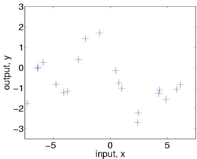
Take a look at the data:
plot(x, y, 'k+', 'MarkerSize', 17)

Now, we compute the predictions for this data using a Gaussian process with
a covariance function being the sum of a squared exponential (SE) contribution
and an independent noise contribution:
covfunc = {'covSum', {'covSEiso','covNoise'}};
To verify how many hyperparameters this covariance function expects:
feval(covfunc{:})
which reurns '2+1', ie two hyperparameters for the SE part (a
characteristic length-scale parameter and a signal magnitude parameter) and a
single parameter for the noise (noise magnitude). We specify the
hyperparameters ell=1.0 (characteristic length-scale),
sigma2f=1.0 (signal variance) and sigma2n=0.01 (noise
variance)
loghyper = [log(1.0); log(sqrt(1.0)); log(sqrt(0.01))]; % this is for figure 2.5(a)
We place 201 test points evenly distributed in the interval [-7.5,
7.5] and make predictions
  xstar = linspace(-7.5,7.5,201)';
  [mu S2] = gpr(loghyper, covfunc, x, y, xstar);
The predictive variance is computed for the distribution of test targets, which
are assumed to be as noisy as the training targets. If we are interested
instead in the distribution of the noise-free function, we subtract the noise
variance from S2
S2 = S2 - exp(2*loghyper(3));
To plot the mean and two standard error (95% confidence), noise-free, pointwise
errorbars:
  hold on
  errorbar(xstar, mu, 2*sqrt(S2), 'g');
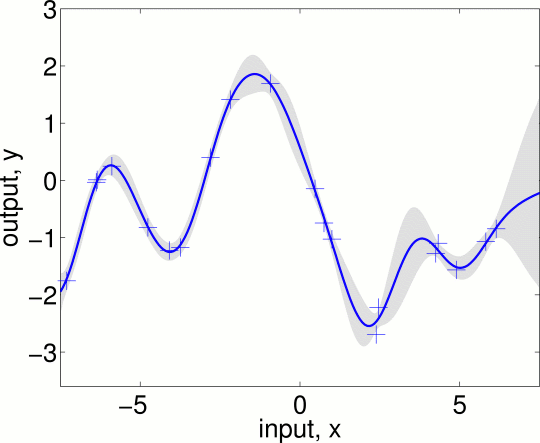
Alternatively, you can also display the error range in gray-scale:
  clf
  f = [mu+2*sqrt(S2);flipdim(mu-2*sqrt(S2),1)];
  fill([xstar; flipdim(xstar,1)], f, [7 7 7]/8, 'EdgeColor', [7 7 7]/8);
  hold on
  plot(xstar,mu,'k-','LineWidth',2);
  plot(x, y, 'k+', 'MarkerSize', 17);
which procudes

reproducing Figure 2.5(a), section 2.3, page 20. Note that the two standard
deviation error bars are for the noise-free function. If you rather want the
95% confidence region for the noisy observations you should not subtract the
noise variance sigma2n from the predictive variances S2. To
reproduce Figs 2.5 (b) and (c) change the log hyperparameters when calling the
prediction program to:
  loghyper = [log(0.3); log(1.08); log(5e-5)];  % this is for figure 2.5(b)
  loghyper = [log(3.0); log(1.16); log(0.89)];  % this is for figure 2.5(c)
respectively. To learn, or optimize the hyperparameters by maximizing the
marginal likelihood using the derivatives from equation (5.9) section 5.4.1
page 114 using minimize.m do:
  loghyper = minimize([-1; -1; -1], 'gpr', -100, covfunc, x, y);
  exp(loghyper)
Here, we initialize the log of the hyperparameters to be all at minus one. We
minimize the negative log marginal likelihood wrt. the log of the
hyperparameters (allowing 100 evaluations of the function (this is
more than adequate)), and report the hyperparameters:
  1.3659
  1.5461
  0.1443
Note that the hyperparameters learned here a close, but not identical to the
log hyperparameters 1.0, 1.0, 0.1 used when generating the data. The
discrepancy is partially due to the small training sample size, and partially
due to the fact that we only get information about the process in a very
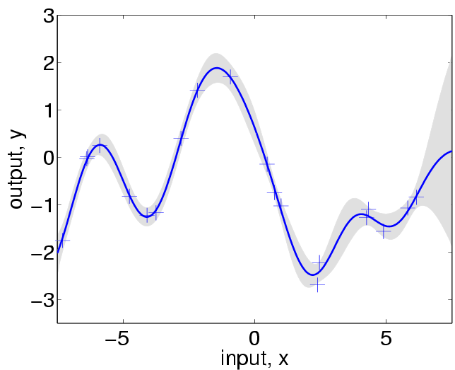
limited range of input values. Predicting with the learned hyperparameters
produces:

which is not very different from the plot above (based on the hyperparameters
used to generate the data). Repeating the experiment with more training points
distributed over a wider range leads to more accurate estimates.
Note, that above we have use the same functional form for the covariance
function, as was used to generate the data. In practise things are seldom so
simple, and one may have to try different covariance functions. Here, we try
to explore how a Matern form, with a shape parameter of 3/2
(see eq. 4.17) would do.
  covfunc2 = {'covSum',{'covMatern3iso','covNoise'}};
  loghyper2 = minimize([-1; -1; -1], 'gpr', -100, covfunc2, x, y);
Comparing the value of the marginal likelihoods for the two models
  -gpr(loghyper, covfunc, x, y)
  -gpr(loghyper2, covfunc2, x, y)
with values of -15.6 for SE and -18.0 for Matern3, shows that
the SE covariance function is about exp(18.0-15.6)=11 times more
probable than the Matern form for these data (in agreement with the data
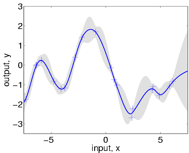
generating process). The predictions from the worse Matern-based model
  [mu S2] = gpr(loghyper2, covfunc2, x, y, xstar);
  S2 = S2 - exp(2*loghyper2(3));
look like this:

Notice how the uncertainty grows more rapidly in the vicinity of data-points,
reflecting the property that for the Matern class
with a shape parameter of 3/2 the stochastic process is not twice mean-square
differentiable (and is thus
much less smooth than the SE covariance function).
3. GPR demo using gpr.m with multi-dimensional input space and
ARD
This demonstration illustrates the use of a Gaussian Process
regression for a multi-dimensional input, and illustrates
the use of automatic relevance determination (ARD). It is based
on Williams and Rasmussen (1996).
You can either follow the example below or run the script demo_gparm.m.
We initially consider a 2-d nonlinear robot arm mapping problem as defined in
Mackay (1992)
f(x_1,x_2) = r_1 cos (x_1) + r_2 cos(x_1 + x_2)
where x_1 is chosen randomly in [-1.932, -0.453], x_2 is chosen randomly in
[0.534, 3.142], and r_1 = 2.0, r_2 = 1.3. The target values are obtained by
adding Gaussian noise of variance 0.0025 to f(x_1,x_2). Following Neal (1996) we add four further inputs, two of which (x_3
and x_4) are copies of x_1 and x_2 corrupted by additive Gaussian noise of
standard deviation 0.02, and two of which (x_5 and x_6) are N(0,1) Gaussian
noise variables. Our dataset has n=200 training points and nstar=200 test
points.
The training and test data is contained in the file data_6darm.mat. The raw training data is
in the input matrix X (n=200 by D=6) and the target
vector y (200 by 1). Assuming that the current directory is
gpml-demo we need to add the path of the code, and load the data:
  addpath('../gpml');    % add path for the code
  load data_6darm
We first check the scaling of these variables using
mean(X), std(X), mean(y), std(y)
In particular we might be concerned if the standard deviation is very different
for different input dimensions; however, that is not the case here so we do not
carry out rescaling for X. However, y has a non-zero mean
which is not appropriate if we assume a zero-mean GP. We could add a constant
onto the SE covariance function corresponding to a prior on constant offsets,
but here instead we centre y by setting:
  offset = mean(y);
  y = y - offset;         % centre targets around 0.
We use Gaussian process regression with a squared exponential covariance
function, and allow a separate lengthscale for each input dimension, as in
eqs. 5.1 and 5.2. These lengthscales (and the other hyperparameters sigma_f
and sigma_n) are adapted by maximizing the marginal likelihood (eq. 5.8)
w.r.t. the hyperparameters. The covariance function is specified by
covfunc = {'covSum', {'covSEard','covNoise'}};
We now wish to train the GP by optimizing the hyperparameters. The
hyperparameters are stored as logtheta = [log(ell_1), log(ell_2),
... log(ell_6), log(sigma_f), log(sigma_n)] (as D = 6), and are
initialized to logtheta0 = [0; 0; 0; 0; 0; 0; 0; log(sqrt(0.1))]. The
last value means that the initial noise variance sigma^2_n is set to 0.1. The
marginal likelihood is optimized using the minimize function.
  logtheta0 = [0; 0; 0; 0; 0; 0; 0; log(sqrt(0.1))];
  [logtheta, fvals, iter] = minimize(logtheta0, 'gpr', -100, covfunc, X, y);
  exp(logtheta)
By doing exp(logtheta) we find that:
  ell_1      1.804377
  ell_2      1.963956
  ell_3      8.884361
  ell_4     34.417657
  ell_5   1081.610451
  ell_6    375.445823
  sigma_f    2.379139
  sigma_n    0.050835
Notice that the lengthscales ell_1 and ell_2 are short indicating that inputs
x_1 and x_2 are relevant to the task. The noisy inputs x_3 and x_4 have longer
lengthscales, indicating they are less relevant, and the pure noise inputs x_5
and x_6 have very long lengthscales, so they are effectively irrelevant to the
problem, as indeed we would hope. The process std deviation sigma_f is similar
in magnitude to the standard deviation of the data std(y) = 1.2186.
The learned noise standard deviation sigma_n is almost exactly equal to the
generative noise level sqrt(0.0025)=0.05.
We now make predictions on the test points and assess the accuracy of these
predictions. The test data is in Xstar and ystar. Recall that
the training targets were centered, thus we must adjust the predictions by
offset:
  [fstar S2] = gpr(logtheta, covfunc, X, y, Xstar);
  fstar = fstar + offset;  % add back offset to get true prediction
We compute the residuals, the mean squared error (mse) and the predictive log
likelihood (pll). Note that the predictive variance for ystar includes
the noise variance, as explained on p. 18.
  res = fstar-ystar;  % residuals
  mse = mean(res.^2)
  pll = -0.5*mean(log(2*pi*S2)+res.^2./S2)
The mean squared error is 0.002489. Note that this is almost equal to the value
0.0025, as would be obtained from the perfect predictor, due to the added noise
with variance 0.0025.
We can also plot the residuals and the predictive (noise-free) variance for
each test case. Note that the order along the x-axis is arbitrary.
  subplot(211), plot(res,'.'), ylabel('residuals'), xlabel('test case')
  subplot(212), plot(sqrt(S2),'.'), ylabel('predictive std deviation'), xlabel('test case')
4. References
- D. J. C. MacKay, A Practical
Bayesian Framework for Backpropagation Networks, Neural Computation 4,
448-472, (1992)
-
R. M. Neal, Bayesian
Learning for Neural Networks, Springer, (1996)
-
C. K. I. Williams and C. E. Rasmussen, Gaussian Processes
for Regression, Advances in Neural Information Processing Systems 8, pp
514-520, MIT Press (1996).
Go back to the web page for
Gaussian Processes for Machine Learning.
Last modified: Mon Mar 27 16:10:14 CEST 2006


