
FORMICA Tutorial
What is FORMICA?
FORMICA is a gui driven system for
the application of advanced ICA algorithms. The primary extensions to
the basic runica program are (1) adaptive source modeling, and (2) the
ability to estimate multiple ICA component models and segment the data
according to model likelihood. Added computational requirements are
handled by parallelizing the algorithm over multiple nodes in a
cluster. The gui is implemented within the MATLAB environment, but the
algorithm processes are spawned and run independently of MATLAB. Matlab
functions are provided to retrieve and process the algorithm output.
When FORMICA is run, a gui is
launched, in which the parameters for the run and computational
resources (e.g. number of processors, etc.) are defined. When the RUN button in pressed, the program schedules a job to run on the cluster
using the number of requested nodes. The job will start when the
requested number of nodes becomes available.
This document will provide a
working knowledge of the use of FORMICA.
The Interface
The FORMICA gui interface is shown
below.
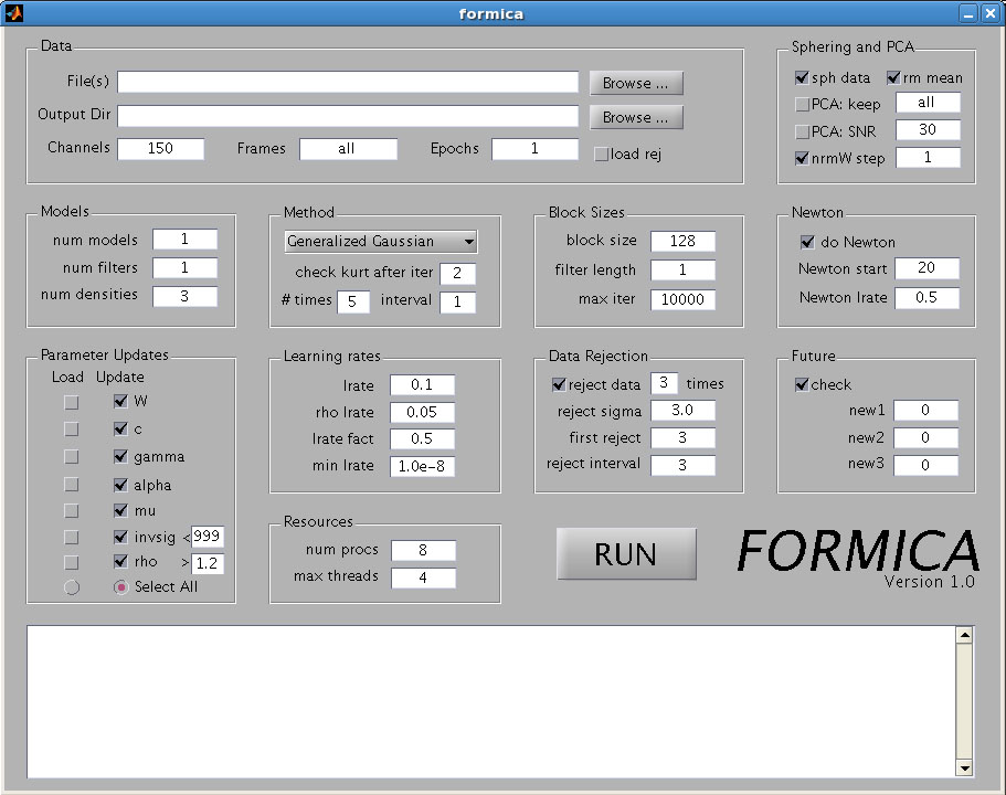
The primary parameter groups
(delimited by boxes) that should be set are: Data, Sphering and PCA,
Models, Method, and Resources. Only the Data parameters are essential
as the default values for the other parameters are usually reasonable.
The parameter groups are described in detail in the following.
- Data
- File(s):
Enter the full path of the data file to be processed. The data should
be stored in floating point format. The Browse button may be used to
locate the file interactively.
- Output Dir: Enter the full
path of the output directory. Again the Browse button can be used to
navigate to a specific directory.
- Channels: Enter the number of channels in the dataset.
- Frames: Enter the number of frames, or time points, in each epoch of the dataset to be processed. The default value of "all" loads all of the data and determines the number of frames from the data size and the number of channels. Usually this field does not need to be set.
- Epochs: Enter the number of continous data segments in the data file. Each epoch should have length equal to the value specified in the Frames field.
- Sphering and PCA
- sph data: Check this box to sphere, or decorrelate, the data prior to running the ICA algorithm. This should usually be checked.
- rm mean: Check this box to remove the mean from each channel. This should also normally be checked.
- PCA: keep: Enter the number of dimensions to retain after sphering. "all" will retain all of the dimensions (equal to the number of channels). If a value less than the number of channels is specified, then the dimensionality will be reduced to that value by eliminating the PCA dimensions with least variance.
- PCA: SNR: Not implemented
- nrmW step: The rows of the unmixing matrix are normalized every iteration, or after then number of iterations specified in this field. Usually the value "1" should be kept.
- Models
- num models: Enter the number of ICA component models to learn from the dataset. It is generally advisable to start with a single model analysis, and possibly add models in subsequent runs.
- num filters: not implemented
- num densities: number of densities in each adaptive source model. Typically "3" is a good value to start with. A higher value subjects the algorithm to overfitting, so the amount of data should be taken into account. For a large amount of data, e.g. "5" densities can be used.
- Method
- Choose the density family within which to adapt the sources. Generalized Gaussian uses Generalized Gaussian densities in the source mixture model. This is usually the best method to use, and doesn't require setting the remaining parameter in this box. The Extended Infomax option chooses the model used by runica. The remaining parameters in the box (explained presently) are only necessary for this option.
- check kurt after: In the Extended Infomax option, this is the iteration to begin evaluating the kurtosis, which is the criterion used to select between two possible source models.
- # times: Check the kurtosis and select density models this number of times.
- interval: Specify the interval in iterations after which to recheck kurtosis and select density models.
- Block sizes
- block size: The size of the block to use in matrix multiplications etc. This only affect the efficiency and speed of the program, not the results.
- filter length: not implemented
- max iter: The maximum number of iterations to be performed if other stopping criteria have not been met.
- Newton
- check do Newton to use the Newton algorithm (faster convergence)
- Newton start: first iteration at which to start using the Newton method (begins with natural gradient)
- Newton lrate: the learning rate for the Newton method (theoretically 1.0 should work, until it gets to the optimum, then this will be scaled back.)
- Parameter updates
- Select the parameters to be updated in the model. Parameters may also be loaded from previous runs from the directory specified in "output directory" as explained below in "Continuing a Run".
- Learning rates
- lrate: The basic learning rate. The learning rate is reduced when the likelihood begins to decrease.
- rho lrate: The learning rate for the shape paramters in the Generalized Gaussian source model.
- lrate fact: The fraction by which the learning rate is reduced after an iteration in which the likelihood decreases.
- min lrate: Stop the algorithm after lrate has been reduced below this value.
- Data rejection
- reject data: Check this box to perform data rejection, and enter the number of times to perform rejection in the field.
- reject sigma: Data points are rejected when their likelihood falls below this number of standard deviations below the average likelihood of the non-rejected data points.
- first reject: The iteration at which to perform the first rejection.
- reject interval: The interval in iterations at which to perform the remaining rejections.
- Future
- For future use.
- Resources
- num procs: The number of processes to run. Each node on the cluster can run up to a certain number of processes (usually 4). The available processes are called slots. User jobs (including MATLAB sessions) are distributed unevenly across the cluster, usually with varying numbers of free slots on each node. The requested processes are distributed across the free slots according to a load scheduling algorithm. Usually the job will be run on several nodes. If the number of slots available is greater than the number of requested procs, the job will start immediately. Otherwise the job waits until enough slots are freed (e.g. by users ending and logging out of MATLAB qlogin sessions.)
- max threads: The maximum number of processes (running as threads) to use on the same node.
Basic ICA (one
model)
- At a matlab prompt, type "/home/jason/formica/formica". This brings up the gui.
- Browse or enter a filtename in Data->File(s) of floating point data, saved by column (as from matlab).
- Enter output directory, e.g. /home/user/newout
- Change number of channels to the number channels in the datafile.
- If doing PCA: check PCA: keep and enter the number of components you want to keep (less than the number of channels.)
- Under Models, if you want to change the number of densities in the source pdf approximation, change "num densities" to the number you want, e.g. 5.
- To do data rejection, make sure reject data is checked, enter number of times, etc. as explained above.
- Under Resources, change "num procs" to the number of processors you want to use (there are 4 per quad-core machine).
- Press "RUN". The white area will display the qsub id number and the output directory.
Multiple models
- Same as for one model, but under Models change "num models" to the number of models you want to learn.
Monitoring
the output
- You can monitor the output of the algorithm using "cat qsub.sh.oXXX" where XXX is the qsub id output in the gui. Doing "watch tail -n 70 qsub.sh.oXXX" should show the last 70 lines of the file, refreshing every 2 seconds. To see which nodes are being used, type "cat qsub.sh.poXXX". The qsub.sh.oXXX and poXXX files should be in your home directory, or in the output directory named in the algorithm.
Loading the
output
- At a matlab prompt type:
[A,varord,LLt,LL,c,W,S,gm,alpha,mu,sbeta,rho,mn,nd,svar] = loaddat3(outdir,nx,nw,num_models,num_mix,max_iter)
where outdir is the output directory (string), nx is the number of channels, nw is the pca reduced dimension (number in pca: keep), num_models is number of models, num_mix is number of mixture source densities, and max_iter is maximum number of iterations for the run. - The main output is the A matrix. This contains the components in the columns. A(:,c,m) is component c of model m. A(:,:,m) is the mixing matrix of model m.
- varord(:,m) is a vector of the indices of the components for model m in variance order. A(:,varord(c,m),m) is the cth largest variance component in model m.
- LLt is a matrix of log likelihoods of the time points for each model. LLt(m,:) is the likelihood time series for model m. [LLmax,LLmod] = max(LLt); gives the index of the most likely model for each time point in LLmod and it's likelihood in LLmax. If LLt(:,t) (and thus LLmax(t)) are zero, then time point t was rejected.
- LL is a length max_iter array that records the overall model log likelihood per sample for each iteration up to when the program stopped, and zeroes filling out the array.
- c is a matrix containing the model centers. c(:,m) is the "center" for model m (after the data mean has been removed). If there is only one model, then c = 0.
- W is the output unmixing matrices, and S is the sphering matrix. W(:,:,m)*S(1:nw,:) is the unmixing matrix for model m (and the pseudoinverse of A(:,:,m)).
- gm, alpha, mu, sbeta, rho are parameters of the source model.
- mn is the original data mean.
- nd is the norm of the update for each component in each model at each iteration. nd(c,m,k) is the norm of the update for component c in model m at iteration k.
- svar is the variance of the
components. svar(c,m) is the variance of component c in model m.
Continuing a run
- Check the "select all" radio button uner Parameter updates,
Load. Put the old output directory in "Output Dir". A new directory
will be created with "_cont" appended to the end.